Much of the work that I do for my PhD is at the confluence of meteorology, optimization, and power systems engineering. I work on incorporating weather data into various long-term power system planning models so that these models design a power grid that is resilient to severe weather events. Optimization is still something I’m relatively new at, but I’ve become increasingly interested in it during my time at Iowa State as an approach to problem solving. As such, I figured it would be worthwhile to write a 3-part blog on optimization and expansion planning, both as a reference for myself and the reader. If nothing else, I hope the reader appreciates optimization not just as a mathematical discipline, but as a framework for approaching life. As humans, we are always trying to optimize something – maybe we are trying to negotiate a higher salary at a job, maybe we are trying to get a restful night sleep, maybe we are trying to break our coffee habit. We are always making decisions, and optimization allows us to take all available information and find the decisions that will yield our desired outcome.
More specifically, optimization is the field of minimizing or maximizing some mathematical function, subject to certain constraints and assumptions. Optimization is widespread throughout power systems engineering and energy trading. For example, the day-ahead and real-time markets use two optimization algorithms: security-constrained unit commitment (SCUC) for the day-ahead market, and security-constrained economic dispatch (SCED) for the day-ahead & real-time markets. The SCUC makes “on/off” generation unit commitment decisions for units within the day-ahead market, while the SCED is responsible for determining the actual dispatch in megawatts for the different units. The SCUC is an integer program and is much more computationally expensive than the SCED, which is a linear program.
Expansion planning is done over multiple decades – not minutes or days like the SCED and SCUC, but it uses the same optimization framework: finding the most efficient/lowest cost method of accomplishing a task. Expansion planning is defined as the process of developing a power plan to meet long-term load projections, subject to certain technical, economic, and political constraints. Much of the material I will use in the next several blogs is adapted from a wonderful paper on the subject: Co-optimization of electricity transmission and generation resources for planning and policy analysis: review of concepts and modeling approaches by Krishnan, Ho, Hobbes, Liu, McCalley, Shahidehpour & Zheng, which was in turn adopted from a 200-page white paper from the same authors discussing the topic in much more detail. Dr. James McCalley is my advisor in the Electrical & Computer Engineering Department at Iowa State and is an expert in optimization and long-term planning, and I highly suggest reading the paper if you are interested in more on the topic. The papers are written for policymakers without a background in electrical engineering, and though they are dense, they are accessible for a general audience.
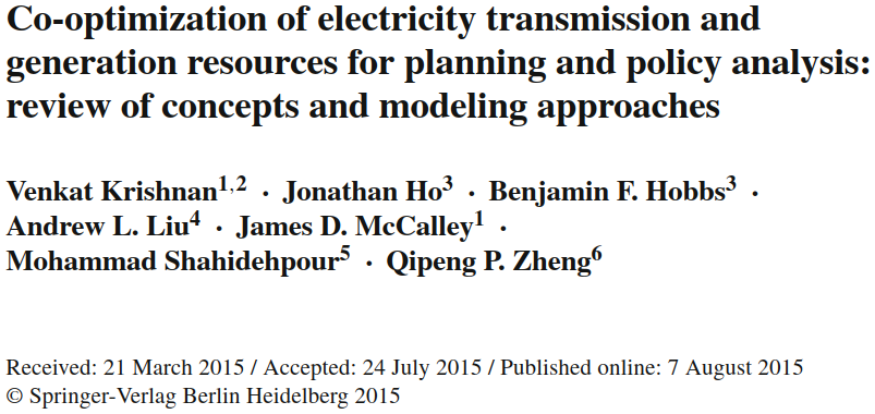
In this blog post, I’ll talk about mathematical optimization (specifically, a type of optimization known as linear programming), give a brief overview of sequential vs. co-optimized expansion planning, and illustrate the superiority of co-optimized expansion planning with a simple example from Krishnan’s paper. In the next blog, I will talk about three different levels of fidelity we use when modeling power flows in an expansion planning model: the “transshipment” model, the ACOPF (alternating current optimal power flow), and the DCOPF (direct current optimal power flow), along with the benefits and drawbacks of each. My final blog will talk about some other major considerations we make in long-term planning, such as the co-optimization of entire sectors, the different timelines and optimization frameworks within a single expansion planning model, and a process known as “anticipatory transmission planning” that is used in industry to predict how generation investments will respond to transmission investments.
Linear Programming
Linear programming was first developed by Soviet mathematician Leonid Kantorovich in his 1939 paper “Mathematical Methods of Organizing and Planning Production.” In the introduction, Kanterovich noted that there are two ways to increase the efficiency of a task – first, by improving the technology needed for that task, and second, by improving the planning and production of that task. The latter had been given very little attention and was the focus of Kantorovich’s work.
The original motivation for Kantorovich’s research was optimizing production schedules for a plywood factory, but linear programming techniques became much more widely used during WWII for a variety of logistics problems. In 1941, Frank Lauren Hitchcock independently discovered linear programming as a method to improve transportation schedules, and in 1947, George Dantzig, a mathematician for the US Air Force, independently formulated a more elegant method of solving linear programming problems known as the Simplex Algorithm. Since WWII, linear programming has gained widespread use for optimizing logistics, planning, and production management across industries. The term “programming” refers not to the use of computers, but as a synonym for “planning” – i.e. “production programming” for creating manufacturing schedules, or “military programming” for allocating resources to support military objectives.
A linear programming problem consists of an objective function, which is the function you are trying to optimize (i.e. – find the minimum or maximum value of), decision variables, which are the variables with values that influence the final output, and constraints, which place limits on the numerical values of these decision variables. The “solution” to a linear programming problem is the unique set of values for each decision variable by which, when that specific combination of variables is put into the objective function, the minimum (or maximum) value of that objective function is reached.
When formulating optimization problems into a mathematical framework, I like to break the problem down into 5 steps:
1. Find out what the problem is asking
2. Identify the decision variables
3. Define the objective function
4. Define the constraints
5. Identify the upper and lower boundaries of the decision variables
Let’s try with the below example.
A school is preparing a trip for 400 students. The company that is providing the transportation has 10 buses of 50 seats each and 8 buses of 40 seats, but it only has 9 drivers available. The rental cost is 800 dollars for a large bus and 600 dollars for a small bus. Calculate how many buses of each type should be used for the trip for the least possible cost.
1. Find out what the problem is asking: Want to find the lowest-cost combination of buses to transport the students
$x_1$: Number of large buses purchased
$x_2$: Number of small buses purchased
Minimize: $C = 800x_1 + 600x_2$
4. Constraints:
Driver limit: $x_1 + x_2 \leq 9$
Student seating requirement: $50x_1 + 40x_2 \geq 400$
Large bus limit: $x_1 \leq 10$
Small bus limit: $x_2 \leq 8$
Non-negativity: $x_1 \geq 0, \quad x_2 \geq 0$
Optimization and linear programming is ubiquitous in our world. FedEx uses it for package delivery, airlines use it to schedule flights, google maps uses it to plan your route. Heck, I use it when I’m grocery shopping!

Linear Programming for Expansion Planning
Needless to say, the mathematical formulation for linear programming in the context of long-term planning is far more detailed and complex than the bus example. However, the framework is the exact same. The constraints for power plans include the physical laws that govern electromagnetism, the operating characteristics of generating units, constraints for different policy pathways, electricity demand projections, and many more. The decision variables are all of the investment or retirement decisions that the model makes. The objective function is the lowest-cost set of generation and/or transmission resources that are needed to meet all of those constraints, such as the locations/size of each generator, the transmission line ratings, the amount of battery storage, etc. It is a remarkably elegant framework for an extraordinarily complex problem.
An expansion planning model is initialized with a network of buses over which transmission lines can connect and generation/load can be added to. This network is typically a simplified representation of the existing power grid so that the planning algorithm is computationally feasible.
Historically, the expansion planning process for generation and transmission occurred sequentially. First, a generation expansion plan (GEP) was created with a “copper plate assumption” (i.e. modeling the generation source as a single node within an electric system, with an unconstrained flow of electricity between components). Second, a transmission expansion plan (TEP) was created by optimizing transmission investments on top of the GEP. This sequential process is also known as “reactive expansion planning” because the transmission investments are created “in response” to generation investments.
Co-optimized Expansion Planning
Unlike reactive expansion planning with sequential GEP and TEP programs, co-optimized expansion planning (CEP) finds an optimal set of generation and transmission lines in a single program.
The Krishnan paper states that co-optimization is important for two reasons. First, generation & transmission can provide the same services. For example, a local thermal power plant can provide dispatchable generation to meet load, while long-distance transmission can import energy from a wind/solar-producing region to do the same. Second, transmission investments will impact the siting of new generation, and the reactive, generation-then-transmission expansion planning that is often undertaken by utilities does not capture this relationship. Co-optimized models can both find where generation or transmission is preferred for providing a certain service (energy, capacity, ancillary services, etc.) and capture the interactions between the two.
An example of the importance of available transmission is the buildout of wind farms over the Interior Northwest. Eastern Montana has a much better wind resource than Central/Eastern Washington, but because Central/Eastern Washington has so much transmission due to the Columbia River hydro system, Central/Eastern Washington has more installed wind generation. However, Montana has begun to close the gap in recent years, and with projects like the North Plains Connector and Southwest Power Pool expanding into the Western United States, I wouldn’t be surprised if Montana overtakes Washington and Oregon in the next decade.
With wind and solar taking up an increasing share of our resource mix – and much more planned to come online in the coming decades, accurately modeling and benefiting from geographical and meteorological diversity will become increasingly more important. So while co-optimized expansion planning has yielded benefits over sequential planning, those benefits may be even greater in the future.
Early Co-optimized Expansion Planning Models
Co-optimized expansion planning models were initially developed in the 60s, and the inclusion of transmission into the generation expansion planning problem was well described in Turvey & Anderson’s 1977 book “Electricity Economics” (see pp. 280-282). However, due to severely limited computational power, early co-optimization algorithms made many simplifications about how power flows on the electric grid. For example, they used a “transshipment” approach for modeling electric power flows, which only respects the power balance constraint at every node and transmission flow limits. It does not actually account for the physical laws that govern the flow of electricity, such as the impedences of each transmission line and voltages at each node. A consequence of this is that it does not model the parallel paths that electricity will take in a network and as a result, it tends to overstate the amount of transmission capacity that is available and understate the amount of transmission capacity needed for investment. Additionally, some of these early models, such as those used in the late 70s under President Carter’s National Coal Utilitization Assessment, treated power plants and transmission lines as continuous variables that could have any non-negative capacity. In reality, transmission lines and power plants are built in discrete sizes. Despite these simplifications, those planning models were useful for anticipating future generation and transmission investment, as they still solved the problem of showing the least cost generation/transmission mix needed to serve demand.
Current Co-optimization Models
Nowadays, planning models have much more computational power available. Though a transshipment approach can still be used to save computational power when needed, models nowadays can model DC load flow approximations or – if the network is relatively small – can explicitly model AC load flows. The models tend to operate within one of two cases (1): high-fidelity models for explicitly modeling individual generation & transmission additions over a small region (such as a utility service territory), or (2) lower-fidelity tools over larger regions that model aggregated investments. The higher fidelity tools are primarily used by those engineering the grid – such as utilities and ISOs – who must have a good grasp on how each generator or substation they add will impact the physical behavior of the bulk power system. The lower-fidelity tools are used more frequently by regulatory bodies and policymakers, as those tools are more useful for anticipating large-scale energy needs.
Co-optimization: A Motivating Example
Krishnan et. al (2015) gives an example with a 3-node network demonstrating how co-optimization yields lower costs than generation or transmission alone. The below figure is adapted from Fig 1 of Krishnan’s paper with extra labeling for clarity, and the values from the below tables are also from the paper.
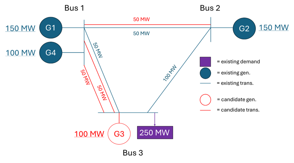
| Unit | Min Capacity (MW) | Max Capacity (MW) | Operating Cost ($/MWh) | Investment Cost ($/year) | Outage Prob. |
| G1 | 0 | 150 | 8 | – | 0.04 |
| G2 | 0 | 150 | 12 | – | 0.04 |
| G3 | 0 | 100 | 9 | 5,000,000 | 0.04 |
| G4 | 0 | 100 | 2 | – | 0.04 |
| Line | From Bus | To Bus | Reactance (pu) | Capacity (MW) | Investment cost ($/year) | Outage Prob. |
| L1 | 1 | 2 | 0.1 | 50 | – | 0.01 |
| L2 | 1 | 3 | 0.1 | 50 | – | 0.01 |
| L3 | 2 | 3 | 0.1 | 100 | – | 0.01 |
| L4 | 1 | 2 | 0.1 | 50 | 3,000,000 | 0.01 |
| L5 | 1 | 3 | 0.1 | 50 | 3,000,000 | 0.01 |
| L6 | 1 | 3 | 0.1 | 50 | 3,000,000 | 0.01 |
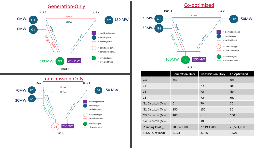
When the network is optimized in generation-only, transmission-only, and co-optimized configurations of Illinois Institute of Technology’s GENTEP model, the below solutions are given. Note how co-optimization provides both lower cost and a lower EENS (expected energy not served). The lower EENS is due to all plants being dispatched to meet load and alleviated congestion between bus 1 & 3, decreasing the risk that the failure of any one plant would cause load shed.
That’s all for this blog. Join me for the next blog on formulating the transshipment, AC Power Flow, and DC Power Flow expansion planning models – I’ll try to get this up in the next few days.